Tutorial: statewide well summary data
python-sa-gwdata has a statewide cache of what we call “summary” data available for you to browse and query.
We will download the relevant data using this package (python-sa-gwdata) – importable as sa_gwdata – and use some other packages for other things:
matplotlib, numpy, pandas - used in the background
[6]:
import sa_gwdata

import pandas as pd
import matplotlib.pyplot as plt
import geopandas as gpd
import contextily as cx
You might get a warning message like this:

If so, you should run this line of code - it will download the summary statewide layer of summary data:
[7]:
sa_gwdata.cache.update()
The data cache will then sit there until you run the update method (same code as above) again to re-download it. About 200 new wells are created each month, so it may or may not be important to you to update it frequently.
(This next step is optional: You can specify the working coordinate reference system (CRS). I’m going to use SA Lambert GDA2020, which is in eastings and northings and covers the whole state. You can pick any!
[8]:
session = sa_gwdata.get_global_session(working_crs="EPSG:8059")
This variable (session), you can either use, or ignore. If you use the module-level functions as shown below, the package will use session in the background.)
Intro to the summary layer
This dataframe covers all wells/drillholes in South Australia:
[9]:
df = sa_gwdata.summary_layer()
df.info()
<class 'geopandas.geodataframe.GeoDataFrame'>
RangeIndex: 361745 entries, 0 to 361744
Data columns (total 82 columns):
 #   Column                Non-Null Count   Dtype
---  ------                --------------   -----
 0   UNIT_NO               361745 non-null  int64
 1   DHNO                  361745 non-null  int64
 2   NAME                  361745 non-null  object
 3   EASTING               361745 non-null  float64
 4   NORTHING              361745 non-null  float64
 5   ZONE                  361745 non-null  int64
 6   LAT                   361745 non-null  float64
 7   LON                   361745 non-null  float64
 8   REF_ELEV              37821 non-null   float64
 9   GRND_ELEV             268204 non-null  float64
 10  HUND                  361745 non-null  object
 11  PARCEL                361745 non-null  category
 12  PARCELNO              361745 non-null  object
 13  PARCELID              361745 non-null  object
 14  STATE                 361745 non-null  category
 15  MAP                   361745 non-null  int64
 16  NUM                   361745 non-null  int64
 17  MAPNUM                361745 non-null  object
 18  STATUS                361745 non-null  category
 19  STAT_DESC             361745 non-null  category
 20  PURPOSE               361745 non-null  category
 21  PURP_DESC             361745 non-null  category
 22  PURPOSE2              361745 non-null  category
 23  PURP2_DESC            361745 non-null  category
 24  PURPOSE3              361745 non-null  category
 25  PURP3_DESC            361745 non-null  category
 26  ANALFULL              361745 non-null  category
 27  PH                    56393 non-null   float64
 28  TDS                   116645 non-null  float64
 29  TDSDATE               115998 non-null  datetime64[ns]
 30  YIELD                 79926 non-null   float64
 31  YIELD_DATE            76865 non-null   datetime64[ns]
 32  WATER_CUT             59071 non-null   float64
 33  DTW                   115098 non-null  float64
 34  SWL                   114432 non-null  float64
 35  SWLDATE               116673 non-null  datetime64[ns]
 36  DRILL_DATE            296216 non-null  datetime64[ns]
 37  LAT_DEPTH             335617 non-null  float64
 38  ORIG_DEPTH            297636 non-null  float64
 39  MAX_DEPTH             343291 non-null  float64
 40  PERMIT_NO             86345 non-null   float64
 41  PERMIT_EX             361745 non-null  object
 42  LOGGEOPHYS            361745 non-null  category
 43  LOGDRILL              361745 non-null  category
 44  LOGGEOL               361745 non-null  category
 45  LOGSTRAT              361745 non-null  category
 46  LOGHYDROSTRAT         361745 non-null  category
 47  LOGGER_DATA           361745 non-null  category
 48  TELEMETRY_DATA        361745 non-null  category
 49  OBSHUND               361745 non-null  category
 50  OBSSEQ                361745 non-null  int64
 51  OBSNUMBER             361745 non-null  object
 52  CLASS                 361745 non-null  category
 53  WW_CLASS              361745 non-null  category
 54  PRIVATE               361745 non-null  category
 55  EC                    116645 non-null  float64
 56  RSWL                  102010 non-null  float64
 57  AQ_MON                361745 non-null  category
 58  PHOTO                 361745 non-null  category
 59  OWNER_CODE            361745 non-null  category
 60  STATE_ASSET           361745 non-null  category
 61  AQ_MONDESC            361745 non-null  category
 62  SUBURB                361745 non-null  category
 63  LGA                   361745 non-null  category
 64  HUNDRED               361745 non-null  category
 65  SW_CATCHMENT          361745 non-null  object
 66  LANDSCAPESA_CODE      361745 non-null  category
 67  NRM_REGION_CODE       361745 non-null  category
 68  PRESCRIBED_WELL_AREA  361745 non-null  category
 69  PRESC_WATER_RES_AREA  361745 non-null  category
 70  CASE_TO               85991 non-null   float64
 71  MIN_DIAM              97043 non-null   float64
 72  TITLE_PREFIX          361745 non-null  category
 73  TITLE_VOLUME          361745 non-null  object
 74  TITLE_FOLIO           361745 non-null  object
 75  TITLE_ID              361745 non-null  object
 76  GRND_ELEV_DEM         361297 non-null  float64
 77  HGUID                 361745 non-null  int64
 78  FTYPE                 361745 non-null  object
 79  NGIS                  361745 non-null  object
 80  LATEST_REF_POINT_TYP  361745 non-null  object
 81  geometry              361745 non-null  geometry
dtypes: category(35), datetime64[ns](4), float64(21), geometry(1), int64(7), object(14)
memory usage: 143.3+ MB
There are 80 columns with varying degrees of reliability or usefulness. The documentation will cover all of them, eventually, but for now let’s focus on a couple.
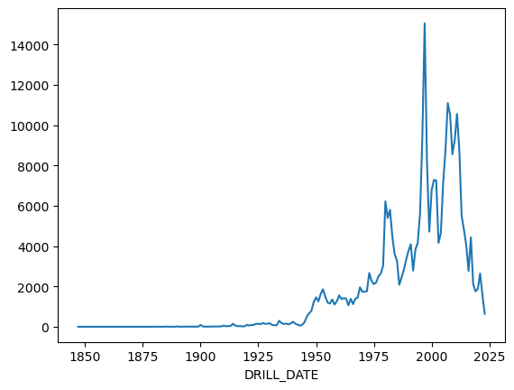
Drilled date
When were most wells drilled?
[24]:
df.groupby(df.DRILL_DATE.dt.year).DHNO.count().plot()
[24]:
<Axes: xlabel='DRILL_DATE'>
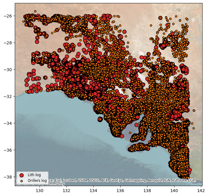
Log availability
Whereabouts are wells with logs located?
[29]:
fig = plt.figure(figsize=(8, 8))
ax = fig.add_subplot(111)
df[df.LOGGEOL == 'Y'].geometry.plot(fc='tab:red', ec='k', marker='o', markersize=80, ax=ax, label='Lith log')
df[df.LOGDRILL == 'Y'].geometry.plot(fc='tab:orange', ec='k', marker='o', markersize=20, ax=ax, label='Drillers log')
cx.add_basemap(ax, source=cx.providers.Esri.WorldImagery, crs=session.working_crs, alpha=0.5)
ax.legend(fontsize='small')
[29]:
<matplotlib.legend.Legend at 0x2a01c9aa4d0>
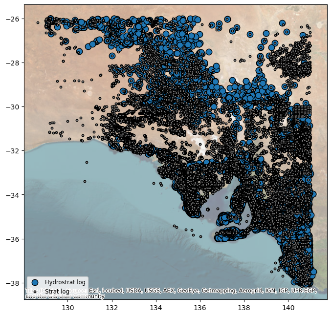
And the below figure compares hydrostrat logs (water-focused) with strat logs (generally more mineral exploration-focused):
[31]:
fig = plt.figure(figsize=(8, 8))
ax = fig.add_subplot(111)
df[df.LOGHYDROSTRAT == 'Y'].geometry.plot(fc='tab:blue', ec='k', marker='o', markersize=80, ax=ax, label='Hydrostrat log')
df[df.LOGSTRAT == 'Y'].geometry.plot(fc='tab:grey', ec='k', marker='o', markersize=10, ax=ax, label='Strat log')
cx.add_basemap(ax, source=cx.providers.Esri.WorldImagery, crs=session.working_crs, alpha=0.5)
ax.legend(fontsize='small')
[31]:
<matplotlib.legend.Legend at 0x2a01c94feb0>
Aquifer monitored codes
These codes show the aquifer which a well is completed in:
[36]:
df.groupby(['AQ_MON']).DHNO.count().sort_values(ascending=False).head(20)
[36]:
AQ_MON
            235758
Thg          20156
Qpm          19168
Qpah         10795
Qpcb          9978
Ty            5025
Nds           4037
Ty(conf)      3560
Qhcks         2797
Ndw           2355
Nnt           1876
Qhck          1733
Tomw(T2)      1636
Ndt           1595
CP-j          1590
Eeb           1557
Qam           1550
Q             1448
Tomw(T1)      1372
Qa            1296
Name: DHNO, dtype: int64
As you can see the majority (235,000) have no aquifer code assigned, since it’s not automatic. The majority of wells with codes are those in the South East (Thg is Gambier Limestone).
More info to come on how to find out more about what those codes mean.
Salinity data - most recent value
The columns TDS and EC have the most recent salinity value, with TDSDATE showing the date:
[11]:
sal_df = df[~pd.isnull(df.EC)]
len(sal_df)
[11]:
116645
So about a third of all wells have at least one salinity measurement:
[20]:
len(sal_df[sal_df.TDSDATE.dt.year >= 2013])
[20]:
12177
And of the wells with salinity observations, only about 10% were measured in the last decade.
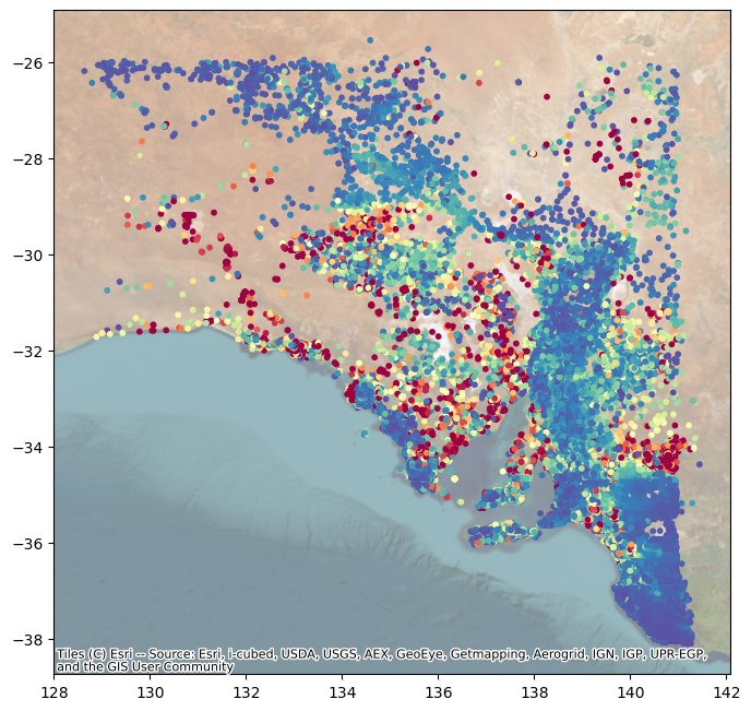
Show a crude visualisation of the variation in salinity:
[49]:
fig = plt.figure(figsize=(8, 8))
ax = fig.add_subplot(111)
sal_df.plot(kind='geo', column='TDS', vmin=100, vmax=30000, markersize=10, ax=ax, cmap='Spectral_r')
cx.add_basemap(ax, source=cx.providers.Esri.WorldImagery, crs=session.working_crs, alpha=0.5)