Tutorial: monitoring networks

This tutorial covers what information is available about monitoring networks.

We will download the relevant data using this package (python-sa-gwdata) – importable as sa_gwdata – and use some other packages for other things:

• matplotlib, numpy, pandas - used in the background

import sa_gwdata

import pandas as pd
import matplotlib.pyplot as plt
import geopandas as gpd
import contextily as cx

This step is optional:

You can specify the working coordinate reference system (CRS). I’m going to use SA Lambert GDA2020, which is in eastings and northings and covers the whole state. You can pick any!

session = sa_gwdata.get_global_session(working_crs="EPSG:8059")

This variable (session), you can either use, or ignore. If you use the module-level functions as shown below, the package will use session in the background. There are some subtle differences which you can see more information about HERE (TODO)

Get a list of monitoring networks

session.networks

{'AW_NP': 'Alinytjara Wilurara Non-Prescribed Area',
 'ANGBRM': 'Angas Bremer PWA',
 'BAROOTA': 'Baroota PWRA',
 'BAROSS_IRR': 'Barossa irrigation wells salinity monitoring',
 'BAROSSA': 'Barossa PWRA',
 'BERI_REN': 'Berri and Renmark Irrigation Areas',
 'BOT_GDNS': 'Botanic Gardens wetlands',
 'CENT_ADEL': 'Central Adelaide PWA',
 'CHOWILLA': 'Chowilla Floodplain',
 'CLARE': 'Clare PWRA',
 'EMLR': 'Eastern Mount Lofty Ranges PWRA',
 'EP_NP': 'Eyre Peninsula Non-Prescribed Area',
 'FAR NORTH': 'Far North PWA',
 'GG_EIZ': 'Golden Grove extractive indust zone',
 'KANGFLAT': 'Kangaroo Flat irrigation wells salinity monitoring',
 'KI_NP': 'Kangaroo Island Non-Prescribed Area',
 'KAT_FP': 'Katarapko Floodplain',
 'LEIGHCK': 'Leigh Creek',
 'LLC_NTH': 'Lower Limestone Coast PWA_North',
 'LLC_STH': 'Lower Limestone Coast PWA_South',
 'LOXTON': 'Loxton - Bookpurnong Irrigation Areas',
 'MALLEE': 'Mallee PWA',
 'MARLA': 'Marla Township',
 'MARNE': 'Marne River and Saunders Creek PWRA',
 'MV_IRR_TDS': 'McLaren Vale  PWA irrigation wells salinity monitoring',
 'MCL_VALE': 'McLaren Vale PWA',
 'MUSGRAVE': 'Musgrave PWA',
 'NOORA_SAW': 'Noora Disposal Basin',
 'NY_NP_NTH': 'Northern & Yorke Non-Prescribed Area - NORTH',
 'NY_NP_STH': 'Northern & Yorke Non-Prescribed Area - SOUTH',
 'NAP_PERCH': 'Northern Adelaide Plains Perched Aquifers',
 'NAP': 'Northern Adelaide Plains PWA',
 'NAP_LIC': 'Northern Adelaide Plains PWA irrigation wells salinity monitoring',
 'PADTH': 'Padthaway PWA',
 'PEAKE': 'Peake, Roby and Sherlock PWA',
 'PIKEMURTHO': 'Pike and Murtho Irrigation Areas',
 'PIKE_FP': 'Pike Floodplain',
 'SAAL_NP': 'SA Arid Lands Non-Prescribed Area',
 'SAMDB_SAW': 'SA Murray Darling Basin - SA Water',
 'SAMDB_NP': 'SA Murray Darling Basin Non-Prescribed Area',
 'SAW_MURTHO': 'SA Water Murtho SIS',
 'SAW_PIKE': 'SA Water Pike SIS',
 'SA_TWS': 'SA Water Town Water Supplies salinity monitoring',
 'SAW_WAIK': 'SA Water Waikerie SIS',
 'SAW_WOOLP': 'SA Water Woolpunda SIS',
 'SE_NP': 'South East Non-Prescribed Area',
 'STHNBASINS': 'Southern Basins PWA',
 'STKILD_MAN': 'St Kilda mangroves',
 'EP_STREAKY': 'Streaky Bay Non-Prescribed Area',
 'TATIARA': 'Tatiara PWA',
 'TINT_COON': 'Tintinara Coonalpyn PWA',
 'WAK_MRK': 'Waikerie Moorook Irrigation Areas',
 'WMLR': 'Western Mount Lofty Ranges PWRA'}

Download wells in the network

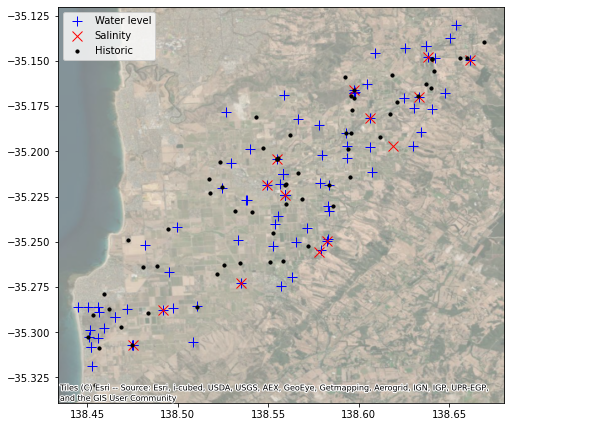
Let’s look at the status of monitoring wells in McLaren Vale PWA

wells = sa_gwdata.search_by_network('MCL_VALE')

The monitoring status of a well is conveyed in these columns:

• swlstatus: water level monitoring status. C = currently monitored

• salstatus: salinity monitoring status. C = currently monitored

“H” means historic i.e. was monitored once, and probably has some data, but not currently monitored.

“N” means “not monitored”, so a similar meaning to “H”, in effect.

wells[['obsnumber', 'obsnetwork', 'swlstatus', 'salstatus']]

	obsnumber	obsnetwork	swlstatus	salstatus
0	WLG036	MCL_VALE	N	H
1	WLG035	MCL_VALE	N	H
2	WLG039	MCL_VALE	H	H
3	WLG038	MCL_VALE	C	H
4	WLG040	MCL_VALE	H	H
...	...	...	...	...
150	WLG156	MCL_VALE	C	N
151	WLG157	MCL_VALE	C	N
152	WLG158	MCL_VALE	C	N
153	NaN	MCL_VALE	N	N
154	WLG190	MCL_VALE	C	N

155 rows × 4 columns

fig = plt.figure(figsize=(8, 8))
ax = fig.add_subplot(111)
wells[wells.swlstatus == 'C'].geometry.plot(color='b', lw=1, marker='+', markersize=100, label='Water level', ax=ax)
wells[wells.salstatus == 'C'].geometry.plot(color='r', lw=1, marker='x', markersize=100, label='Salinity', ax=ax)
historic = (wells.swlstatus != "C") & (wells.salstatus != "C")
wells[historic].geometry.plot(color='k', marker='o', markersize=10, label='Historic', ax=ax)
ax.legend()

cx.add_basemap(ax, source=cx.providers.Esri.WorldImagery, crs=session.working_crs, alpha=0.5)

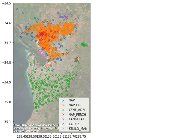
Download more than one network at once

Let’s now download all the Adelaide Plains monitoring networks in one go, and colour the wells by the network they are in.

wells = sa_gwdata.search_by_network(
    'NAP', 'NAP_LIC', 'NAP_PERCH', 'CENT_ADEL', 'GG_EIZ', 'STKILD_MAN', 'KANGFLAT'
)

fig = plt.figure(figsize=(8, 8))
ax = fig.add_subplot(111)

for network in wells.obsnetwork.unique():
    wells[wells.obsnetwork == network].geometry.plot(marker='x', lw=1, ax=ax, label=network)

ax.legend()
cx.add_basemap(ax, source=cx.providers.Esri.WorldImagery, crs=session.working_crs, alpha=0.5)