Tutorial: finding wells

We’re going to try and find some wells!

We will download the relevant data using this package (python-sa-gwdata) – importable as sa_gwdata – and use some other packages for other things:

• matplotlib, numpy, pandas - used in the background

import sa_gwdata

import pandas as pd
import matplotlib.pyplot as plt
import geopandas as gpd
import contextily as cx

(This next step is optional: You can specify the working coordinate reference system (CRS). I’m going to use SA Lambert GDA2020, which is in eastings and northings and covers the whole state. You can pick any!

session = sa_gwdata.get_global_session(working_crs="EPSG:8059")

This variable (session), you can either use, or ignore. If you use the module-level functions as shown below, the package will use session in the background)

Search for wells by suburb

Where do we start? Let’s download a list of all wells in Semaphore as a start.

wells = sa_gwdata.search_by_suburb("semaphore")

If you have geopandas installed, this will return you a geopandas.GeoDataFrame object, which already contains spatial points for the wells in the geometry column.

wells

	dhno	lat	lon	mapnum	unit_no	max_depth	aq_mon	swl	tds	class	...	latest_open_date	name	drill_date	purp_desc	stat_desc	yield	latest_yield_date	permit_no	replaceunitnum	geometry
0	27451	-34.835571	138.483647	652800323.0	6528-323	6.71	Qhcks	5.49	671.0	WW	...	1934-09-06	NaN	NaN	NaN	NaN	NaN	NaN	NaN	NaN	POINT (138.48365 -34.83557)
1	27452	-34.833056	138.484522	652800324.0	6528-324	5.18	Qhcks	NaN	799.0	WW	...	1934-09-28	NaN	NaN	NaN	NaN	NaN	NaN	NaN	NaN	POINT (138.48452 -34.83306)
2	27455	-34.837983	138.479954	652800327.0	6528-327	NaN	Qhcks	1.22	1556.0	WW	...	1934-09-01	TODD"S RESERVE	1934-09-01	NaN	NaN	NaN	NaN	NaN	NaN	POINT (138.47995 -34.83798)
3	27461	-34.837697	138.487967	652800333.0	6528-333	6.10	Qhcks	2.44	1145.0	WW	...	1967-11-13	NaN	NaN	DOM	OPR	NaN	NaN	NaN	NaN	POINT (138.48797 -34.83770)
4	27462	-34.836557	138.485530	652800334.0	6528-334	6.10	Qhcks	3.05	670.0	WW	...	1967-11-13	NaN	NaN	DOM	OPR	NaN	NaN	NaN	NaN	POINT (138.48553 -34.83656)
...	...	...	...	...	...	...	...	...	...	...	...	...	...	...	...	...	...	...	...	...	...
139	331684	-34.838582	138.488233	652802983.0	6528-2983	5.80	NaN	3.20	NaN	WW	...	2019-11-20	NaN	2019-11-20	DOM	NaN	0.4	2019-11-20	354724.0	NaN	POINT (138.48823 -34.83858)
140	332207	-34.837590	138.486967	652802985.0	6528-2985	5.80	NaN	0.00	NaN	WW	...	2019-11-20	NaN	2019-11-20	DOM	NaN	0.4	2019-11-20	354882.0	NaN	POINT (138.48697 -34.83759)
141	353537	-34.843205	138.486937	652803031.0	6528-3031	2.50	NaN	NaN	NaN	WW	...	2020-12-17	NaN	2020-12-17	MON	NaN	NaN	NaN	389634.0	NaN	POINT (138.48694 -34.84320)
142	353538	-34.842472	138.487761	652803032.0	6528-3032	2.50	NaN	NaN	NaN	WW	...	2020-12-17	NaN	2020-12-17	MON	NaN	NaN	NaN	389635.0	NaN	POINT (138.48776 -34.84247)
143	360259	-34.844161	138.483252	652803069.0	6528-3069	3.00	NaN	NaN	NaN	WW	...	NaN	NaN	NaN	NaN	NaN	NaN	NaN	NaN	NaN	POINT (138.48325 -34.84416)

144 rows × 41 columns

wells.info()

<class 'geopandas.geodataframe.GeoDataFrame'>
RangeIndex: 144 entries, 0 to 143
Data columns (total 41 columns):
 #   Column             Non-Null Count  Dtype
---  ------             --------------  -----
 0   dhno               144 non-null    int64
 1   lat                144 non-null    float64
 2   lon                144 non-null    float64
 3   mapnum             144 non-null    float64
 4   unit_no            144 non-null    object
 5   max_depth          142 non-null    float64
 6   aq_mon             136 non-null    object
 7   swl                103 non-null    float64
 8   tds                121 non-null    float64
 9   class              144 non-null    object
 10  title_prefix       134 non-null    object
 11  title_volume       134 non-null    object
 12  title_folio        134 non-null    object
 13  hund               144 non-null    object
 14  parcel             134 non-null    object
 15  parcelno           134 non-null    object
 16  plan               142 non-null    object
 17  planno             142 non-null    object
 18  pwa                144 non-null    object
 19  nrm                144 non-null    object
 20  logdrill           144 non-null    object
 21  litholog           144 non-null    object
 22  chem               144 non-null    object
 23  water              144 non-null    object
 24  sal                144 non-null    object
 25  obswell            144 non-null    object
 26  stratlog           144 non-null    object
 27  hstratlog          144 non-null    object
 28  latest_swl_date    103 non-null    object
 29  latest_sal_date    121 non-null    object
 30  latest_open_depth  138 non-null    float64
 31  latest_open_date   142 non-null    object
 32  name               3 non-null      object
 33  drill_date         134 non-null    object
 34  purp_desc          106 non-null    object
 35  stat_desc          33 non-null     object
 36  yield              113 non-null    float64
 37  latest_yield_date  112 non-null    object
 38  permit_no          135 non-null    float64
 39  replaceunitnum     5 non-null      object
 40  geometry           144 non-null    geometry
dtypes: float64(9), geometry(1), int64(1), object(30)
memory usage: 46.2+ KB

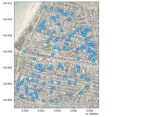
Plot these wells with a background map:

fig = plt.figure(figsize=(8, 8))
ax = fig.add_subplot(111)
wells.geometry.plot(fc='turquoise', ec='b', marker='o', markersize=100, ax=ax)
cx.add_basemap(ax, source=cx.providers.Esri.WorldImagery, crs=session.working_crs, alpha=0.5)

The field “aq_mon” contains data on which aquifer the wells is completed in:

wells.aq_mon.fillna("NA").value_counts()

Qhcks         132
NA              8
Qhck            2
Tomw(T1)        1
Qhcks+Qpah      1
Name: aq_mon, dtype: int64

There’s only one well monitoring the T1 aquifer so let’s expand our search to include nearby suburbs.

wells = pd.concat(
    [
        sa_gwdata.search_by_suburb(suburb) for suburb in
        ("semaphore", "semaphore south", "semaphore park", "ethelton", "largs bay", "birkenhead")
    ]
)

wells.aq_mon.fillna("NA").value_counts()

Qhcks         647
Qhck          359
NA             50
Qpah           41
Tomw(T1)        5
Qhcks+Qpah      1
Tomw(T2)        1
Name: aq_mon, dtype: int64

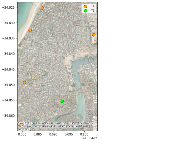
That’s better

t_wells = wells[wells.aq_mon.isin(["Tomw(T1)", "Tomw(T2)"])]

fig = plt.figure(figsize=(8, 8))
ax = fig.add_subplot(111)
t_wells[t_wells.aq_mon == "Tomw(T1)"].geometry.plot(fc='orange', ec='r', marker='o', markersize=100, ax=ax, label="T1")
t_wells[t_wells.aq_mon == "Tomw(T2)"].geometry.plot(fc='lime', ec='green', marker='o', markersize=100, ax=ax, label="T2")
cx.add_basemap(ax, source=cx.providers.Esri.WorldImagery, crs=session.working_crs, alpha=0.5)
ax.legend()

<matplotlib.legend.Legend at 0x234c2a8d8d0>

t_wells

	dhno	lat	lon	mapnum	unit_no	max_depth	aq_mon	swl	tds	class	...	stat_desc	yield	latest_yield_date	permit_no	replaceunitnum	geometry	obsnumber	obsnetwork	swlstatus	salstatus
125	206608	-34.832417	138.482484	652802547.0	6528-2547	154.00	Tomw(T1)	NaN	NaN	Strat	...	NaN	NaN	NaN	NaN	NaN	POINT (138.48248 -34.83242)	NaN	NaN	NaN	NaN
5	27545	-34.849275	138.480715	652800417.0	6528-417	103.02	Tomw(T1)	9.14	7600.0	WW	...	BKF	NaN	NaN	NaN	NaN	POINT (138.48072 -34.84928)	NaN	NaN	NaN	NaN
9	27582	-34.863053	138.479540	652800454.0	6528-454	173.13	Tomw(T1)	9.75	3027.0	WW	...	UKN	17.68	1951-07-20	NaN	NaN	POINT (138.47954 -34.86305)	NaN	NaN	NaN	NaN
13	27587	-34.855317	138.492849	652800459.0	6528-459	198.12	Tomw(T2)	5.18	2792.0	WW	...	BKF	19.32	1971-08-23	254671.0	NaN	POINT (138.49285 -34.85532)	NaN	NaN	NaN	NaN
0	27150	-34.825235	138.486454	652800003.0	6528-3	92.96	Tomw(T1)	3.05	1385.0	PW	...	ABD	1.00	1931-12-01	NaN	NaN	POINT (138.48645 -34.82524)	NaN	NaN	NaN	NaN
75	51506	-34.833889	138.503017	662804537.0	6628-4537	108.20	Tomw(T1)	3.66	2585.0	WW	...	NaN	15.15	1960-03-16	NaN	NaN	POINT (138.50302 -34.83389)	NaN	NaN	NaN	NaN

6 rows × 45 columns

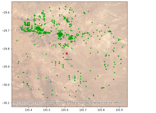
Searching by location and radius

Let’s look for wells near a mine like Prominent Hill:

using a radius search of 30 km

lat = -29.827870
lon = 135.610701
radius_km = 30

wells = sa_gwdata.search_by_radius(lat, lon, radius_km)

wells

	dhno	lat	lon	mapnum	max_depth	drill_date	swl	tds	stat_desc	class	...	permit_no	yield	latest_yield_date	aq_mon	obsnumber	obsnetwork	swlstatus	salstatus	replaceunitnum	geometry
0	9758	-30.005110	135.399494	593700062.0	30.78	1962-05-08	21.64	743.0	ABD	WW	...	NaN	NaN	NaN	NaN	NaN	NaN	NaN	NaN	NaN	POINT (135.39949 -30.00511)
1	9759	-30.025724	135.413100	593700063.0	33.53	1962-05-02	NaN	NaN	ABD	WW	...	NaN	NaN	NaN	NaN	NaN	NaN	NaN	NaN	NaN	POINT (135.41310 -30.02572)
2	9820	-30.024907	135.455566	593700124.0	130.00	1981-01-01	NaN	NaN	UKN	MW	...	NaN	NaN	NaN	NaN	NaN	NaN	NaN	NaN	NaN	POINT (135.45557 -30.02491)
3	332884	-30.053247	135.479734	593700537.0	65.50	2019-12-02	54.00	6977.0	OPR	WW	...	342340.0	1.00	2019-12-02	NaN	NaN	NaN	NaN	NaN	NaN	POINT (135.47973 -30.05325)
4	9968	-29.871678	135.345502	593800010.0	89.47	1930-01-01	77.87	7609.0	NIU	WW	...	NaN	0.42	1952-07-30	K-c(unconf)	NaN	NaN	NaN	NaN	NaN	POINT (135.34550 -29.87168)
...	...	...	...	...	...	...	...	...	...	...	...	...	...	...	...	...	...	...	...	...	...
979	371260	-29.976768	135.654835	603800689.0	351.10	2006-10-14	NaN	NaN	NaN	MW	...	NaN	NaN	NaN	NaN	NaN	NaN	NaN	NaN	NaN	POINT (135.65484 -29.97677)
980	371261	-29.960878	135.623841	603800690.0	70.00	2006-10-22	NaN	NaN	NaN	MW	...	NaN	NaN	NaN	NaN	NaN	NaN	NaN	NaN	NaN	POINT (135.62384 -29.96088)
981	371262	-29.964527	135.654839	603800691.0	96.00	2006-11-21	NaN	NaN	NaN	MW	...	NaN	NaN	NaN	NaN	NaN	NaN	NaN	NaN	NaN	POINT (135.65484 -29.96453)
982	371263	-29.968547	135.686714	603800692.0	86.00	2006-11-18	NaN	NaN	NaN	MW	...	NaN	NaN	NaN	NaN	NaN	NaN	NaN	NaN	NaN	POINT (135.68671 -29.96855)
983	371264	-29.981998	135.702844	603800693.0	117.00	2006-11-20	NaN	NaN	NaN	MW	...	NaN	NaN	NaN	NaN	NaN	NaN	NaN	NaN	NaN	POINT (135.70284 -29.98200)

984 rows × 36 columns

fig = plt.figure(figsize=(8, 8))
ax = fig.add_subplot(111)
wells.geometry.plot(fc='lime', ec='green', marker='o', markersize=10, ax=ax)
cx.add_basemap(ax, source=cx.providers.Esri.WorldImagery, crs=session.working_crs, alpha=0.5)

Let’s also put the search point on this map so we can see what happened

search_df = pd.DataFrame({'lat': [lat], 'lon': [lon]})
search_pts = gpd.GeoDataFrame(
    search_df, crs="EPSG:4326", geometry=gpd.points_from_xy(search_df.lon, search_df.lat)
).to_crs(session.working_crs)

search_pts.geometry.plot(marker='*', c='red', markersize=100, label='Search point', ax=ax, aspect=1)

ax.figure

<Figure size 432x288 with 0 Axes>

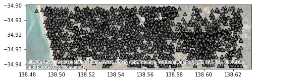
Searching by a rectangle

Let’s search for wells in a rectangle - shall we try to retrieve a cross section of wells across the Adelaide Plains below the Para Fault?

I’ll need to get the latitude and longitude of the:

• south-western corner i.e. bottom left (min latitude and min longitude) and the

• north-eastern corner i.e. top right (max latitude and max longitude)

ne_corner = -34.901291, 138.484388
sw_corner = -34.941296, 138.625417

wells = sa_gwdata.search_by_rect(ne_corner, sw_corner)
fig = plt.figure(figsize=(8, 8))
ax = fig.add_subplot(111)
wells.geometry.plot(fc='grey', ec='black', marker='^', markersize=50, ax=ax)
cx.add_basemap(ax, source=cx.providers.Esri.WorldImagery, crs=session.working_crs, alpha=0.5)